During my final semester at Cornell University, I took Autonomous Mobile Robots with Professor Kress-Gazit, which was hands down my favorite course I took at Cornell. This course gives an overview of the challenges and techniques used for creating autonomous mobile robots. Topics include sensing, localization, mapping, path planning, motion planning, obstacle and collision avoidance, and multi-robot control. Throughout the course, classical localization, mapping, path planning and motion planning algorithms were introduced during lecture, giving a theory based understanding of these algorithms. Then, each week, we wrote and implemented these algorithms from scratch in MATLAB. Below is a brief overview of everything written and implemented from scratch, with a few examples provided.
Localization:
- Dead reckoning
- Probabilistic map-based localization
- (Extended) Kalman Filtering
- Particle Filtering
Mapping:
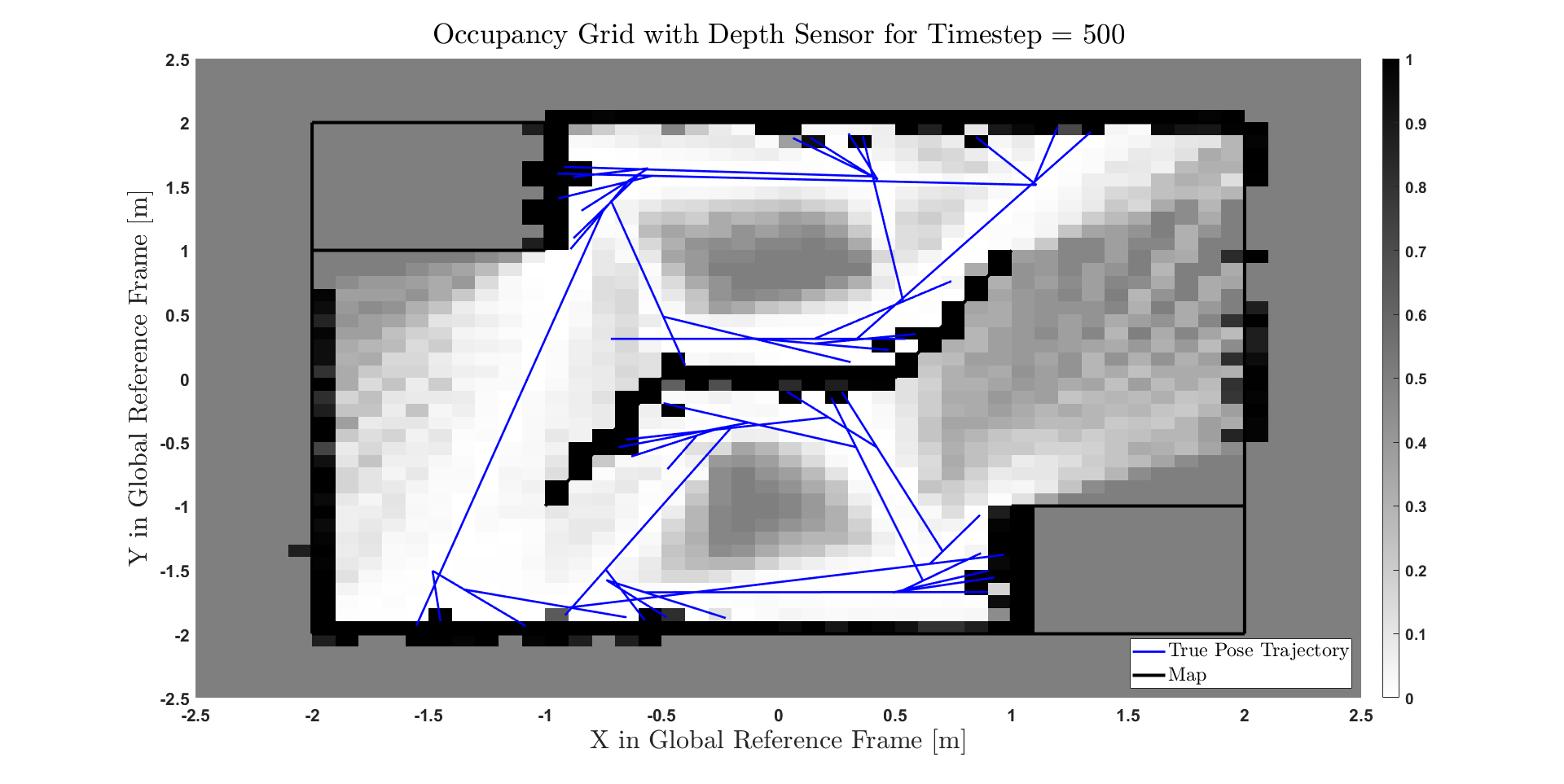
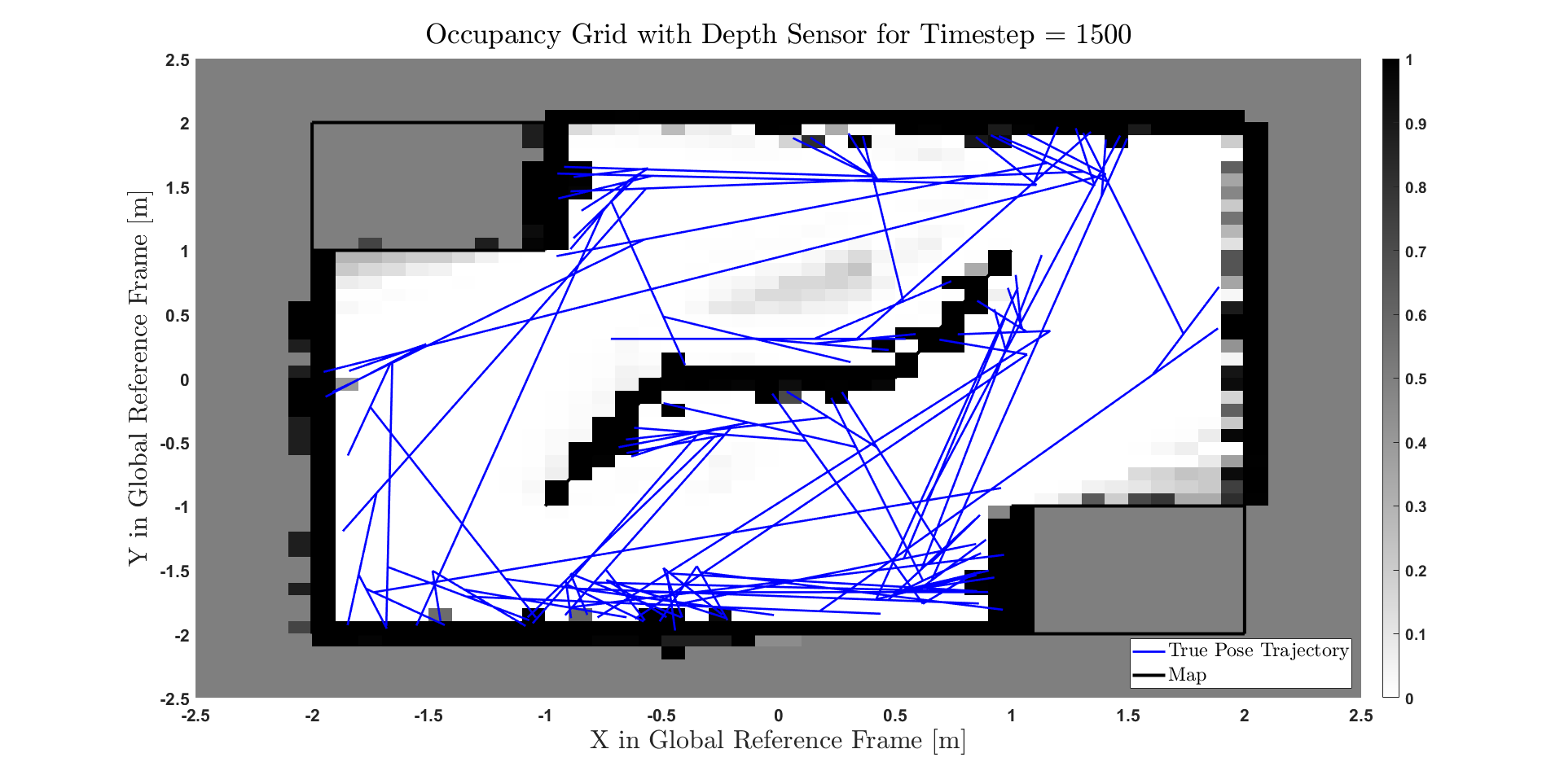
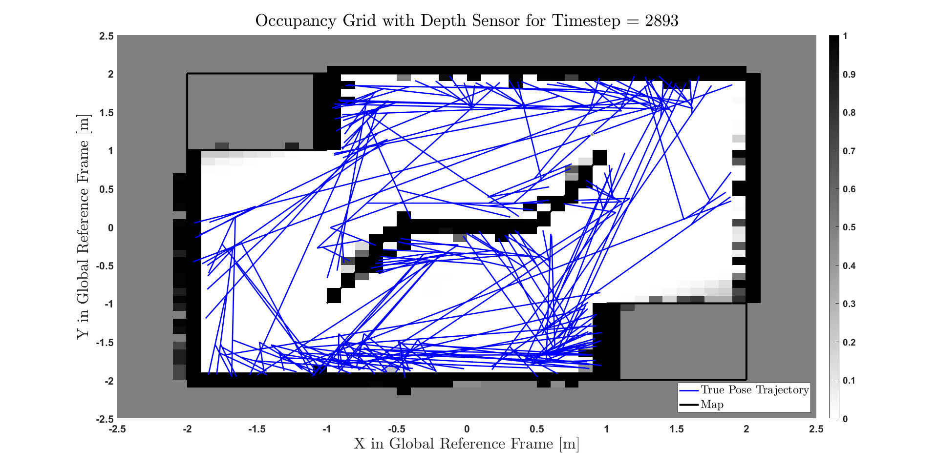
- Occupancy Grid (depth sensor)
- Occupancy Grid (bump sensor)
Motion Plannning:
- Potential functions
- Roadmaps
- RRT’s
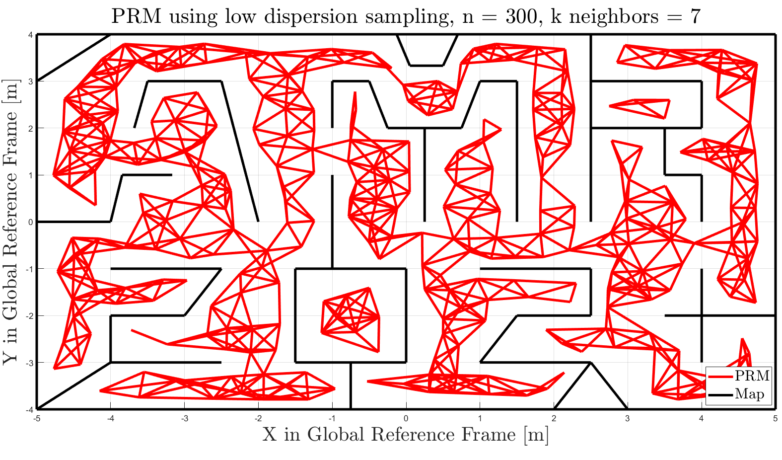
- PRM’s
Final Competition
In the final competition, students were placed in groups of 2 or 3 and tasked with developing a control algorithm for a robot in a simulator to:
- Localize itself (ie. initialize the robot’s starting position, localize the robot as it moves about the environment and avoid hitting obstacles)
- Navigate to as many of the given waypoints as possible.
The robot has information about the map, and has a list of waypoints. Thus, the main task was to perform the localization and the motion planning, and execute the navigation.
Summary of Approach
For initial localization of the robot, we rotated the robot 360 degrees and utilized a custom built Particle Filter (PF) along with the data collected in that spin. We chose to use a PF for the initial localization because it was known that the robot would be starting on a waypoint, and thus the initial particle set could consist of particles on the waypoints with varying headings. While navigating, we used an Extended Kalman Filter (EKF) with only depth data. We chose to use an EKF because when the initial location guess is good, an EKF is almost always able to localize the robot, and we can also quantify the uncertainty in the EKF’s pose estimate using the sigma matrix. When the EKF’s pose estimate reached an unacceptable uncertainty level, we chose to re-localize the robot using one of two possible “emergency” Particle Filter re-localization techniques. The first emergency PF has a particle set of evenly spaced points within a 1 meter grid around the most recent pose estimate with varying headings. We found this technique to be useful in re-localizing the robot when the covariance in x and y was very large. For situations with slightly smaller x and y covariance, or where the covariance in theta exceeded a threshold, we used a similar technique to the initial PF localization algorithm, in which the robot would spin and collect data, and run a PF with the initial particle set located on the most recent pose guess, with varying headings.
For motion planning, we used a k nearest neighbor PRM with low dispersion sampling, because we would only have to generate the roadmap once at the beginning of the script, and the roadmap produced using this sampling method is quite sparse, meaning that we do not require many nodes to cover the entire map. Additionally, it only requires running dijkstra’s once at the beginning of each new path to a new waypoint. To decide the order of waypoints (both extra credit (EC) and normal) we were to travel to, we used a Travelling Salesman Problem (TSP) solver made by Joseph Kirk, making some slight modifications to tailor his script for our application. We used the TSP algorithm because we wanted to achieve the shortest possible total path to all the waypoints.
For more detail, please see the final competition report below.